
1. Modular Semantic Analysis
Todo
How are results consolidated?
Complete overview over
*_Resultsdata structures, in particular, add values.In local mode, where do we get the interprocedural results Andreas is talking about? A: per SSI node, for example:
get_global_values()Inline TODO
Modular Semantic Analysis (MSA) will have multiple modes, of which only the first is implemented. You can see an overview of the basic approach on the right side.

Figure 1.1 An overview of the different analyses in FSPTA.
1.1. Analysis mode: Function-By-Function or Local
In this mode, each routine is analyzed in isolation. Almost no information is propagated from other routines to the analyzed routine, except information derived
from contracts and external specifications, and
from several interprocedural analysis steps (e.g. “called function is pure”)
The Function-By-Function analysis mode is intended to find “interesting” findings with respect to the investigated error categories. It is therefore expected to be fast and might be unsound: it might skip true positives, but reports not too many false positives either. It can apply heuristics in its error checks to achieve this task.
For each routine, the analysis performs the following steps.
Perform basic intraprocedural analyses, including
(local) pointer analysis
creation of SSA/SSI form
numerical analyses like range computation
symbolic expression
Execute configured semantic checks (see library
libSemanticChecks)
See fscs_analysis.cpp in libIntegrated for creation of basic analyses
for MSA.
1.1.1. Results and data structures of different analyses
Analysis results are passed between the different analysis stages through three result
types: Permanent_Results, Interprocedural_Results, and Local_Results.
Permanent_Resultsholds the analysis configuration, aGlobal_Object_Manager, and a list ofInterprocedural_Results.Interprocedural_Resultscontain the call graph (the initial approximated one as well as a final refined one), and twoInterprocedural_Routine_Results, which contain the following results.Interprocedural_Control_Flow_ResultsInterprocedural_Data_Flow_ResultsInterprocedural_Pointer_ResultsInterprocedural_Numerical_Results
Local_Resultslink toPermanent_Results,Interprocedural_Results, and the following five results.Local_Control_Flow_ResultsUnreachable blocks and locally caught exceptions (no control flow graph)Local_Data_Flow_ResultsSSI graph (i.e., data flow graph between SSI nodes), modification side effects (TODO: what is this exactly?), use side effects (TODO: what is this exactly?)Local_Pointer_ResultsMay-alias relation between two pointer targets.Local_Numerical_ResultsNot yet implementedLocal_Relational_Values_ResultsRelations that hold at the beginning of a basic block. Relations are represented as Relational_Value which is NOT a Value.
For SSI nodes, analysis values can also be obtained by
FSPTA::SSI_Node::get_local_values(),
returning a reference to the instance of Analysis_Values associated with the node.
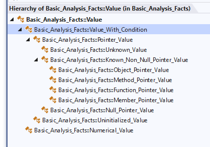
Figure 1.2 FSPTA value types (except the ones that do not inherit Analysis_Value).
1.1.2. Interprocedural Base Analysis
All interprocedural base analyses implement the interface
FSPTA::Interprocedural_Analysis and store their results as Permanent_Results.
This phase is based on the RCI technique and follows the four phases described
in the paper.
Local_Analysis_And_Summary_Extraction(part of phase 1 in RCI)Determine control-flow, data-flow, pointer and numerical results by runningstd_local_analysison an overapproximated call graph, i.e., by looking at every routine in isolation and generating summaries in terms of symbolic values from these results.Separate_Bottom_Up_phase(part of phase 1 in RCI)Propagate symbolic values found in previous analysis bottom up, i.e., compute transitive closure of summaries and global modifications (what part of the heap is untouched by a routine). Resolve symbolic values if possible.RCI_Top_Down_Phase(phase 2 and 3 in RCI)Propagate concrete values to routine entries and inside methods top-down to resolve remaining symbolic values with concrete values.
1.1.3. Intraprocedural Analysis
The various intraprocedural analyses can either run once (linear) or run until a fixed point is reached, i.e., until the current run did not produce any change.
fscs_analysis#std_local_analysis utilizes the following intraprocedural analyses.
Their options and their context (linear or fixed point) depend on various settings.
Figure 1.1 shows their order and their context.
Local_Exception_AnalysisComputes which blocks throw or catch which exceptions.Local_FSPTAFlow-sensitive pointer analysis. Computes points-to sets for all pointer targets as well as data and control flow information. Can perform alias analysis. Based on this PhD thesis.Local_Interval_AnalysisIs going to be merged with Range_Analysis – currently, does nothing.Basic_Local_Control_Flow_AnalysisRefines call graph by using pointer analysis results.Range_AnalysisComplete abstract interpreter (computes its own fixed point, uses simple interval domain together with symbolic expressions and disjunctive states).Condition_AnalysisCombination of multiple analyses, computes its own fixed point.Reset_Alias_Annotationsresets all alias annotations s.t. the next analysis can compute the correct ones.Local_FSPTAwith alias analysis.Local_Node_Condition_Analysisinfers conditions for the existence of nodes or abstract nodes, e.g, only if \(p=q\).Remove_Impossible_Valuesclean-up step that removes impossible values (artefacts of previous analyses).
Symbolic_Access_AnalysisUse abstract interpretation with symbolic expression domain to refine reachable states, distinguish vales that may contain 0 from those that do not, and relational “values” for direct nodes.
1.1.4. Analysing a routine locally in Function-By-Function mode
On the C++ side, the library libSemanticChecks contains implementations of checks
for each supported semantic check (like null-deref, overflow, …) of modular semantic
analysis. The checks can, for each analyzed routine \(r\),
use local results for \(r\) coming from the basic analysis, obtained via
FSPTA::Local_Resultsinstanceadditionally run their own custom analysis for \(r\).
Results are generated by creating Semantic_Checks::Issue instances (see
check.h in libSemanticChecks)
Note:
The corresponding library for error checks in FIPTA is libErrorChecks.
1.2. Data-Flow Representation
To represent the data flow, Modular Semantic Analysis supports two approaches: SSA and SSI. SSI creates more nodes but may help to achieve higher precision.
1.2.1. Nodes in the data-flow graph
We distinguish data-flow nodes and operation nodes. Data-flow nodes represent the typical action on a certain memory location at a certain position in the code, whereas operation nodes represent operations like casts, roughly similar to LIR instruction types.
Types of data-flow nodes:
basic nodes: definition, use, deref_use, postcall, precall, address
block nodes (SSA): entry, exit, uninit, phi_argument, phi_definition
block nodes (SSI): same as for SSA, plus sigma_argument, sigma_definition
A dereferencing use node is a special case of a use node and provides a link to the nodes created for the pointer targets. Precall nodes are used to represent data-flow going into a call; there are precall nodes for the arguments and a placeholder precall node for the use side effects (we only deal with data-flow side effects here, i.e. accessing non-local objects; other side effects are not represented by data-flow nodes). Postcall nodes represent the data-flow coming out of a call; there is a placeholder postcall node for the definition side effects. Taking the address of an object is also represented with a data-flow node, while taking a function’s address is represented with an operation node.
Phi and sigma nodes are split into their effects at the end of the preceding block(s) and the start of the next block(s). The arguments of a phi node represent use-like nodes at the end of branches, while the definition part of a phi node is a def-like node at the beginning of the join block. Likewise, a sigma node has a single argument at the end of the split block and a definition node at the beginning of each branch.
1.2.2. Edges in the data-flow graph
Edges connect nodes in the data-flow graph, available both in data-flow direction (e.g. from def to use of same object, or from RHS to LHS of an assignment, or from operands into the operation) and also against data-flow direction.
For an edge from the reaching definition to a data-flow node, we currently
enforce that the source and target node of such an edge refer to the exact
same object. Possible influences on the data-flow to the target node through
other objects are represented as Alias_Definition points along the edge.
These cover especially the case of pointer-indirect definitions in between
the reaching definition and the node, but also the possible influence from
definition side effects of a call in between. In contrast to FIPTA,
the alias definitions do not involve abstract nodes (see below), but instances
of them (or, in the case of weak updates for array elements, those weak update
nodes). The alias definitions could also be used for other types of aliasing,
e.g. union members.
We also store def-def edges, albeit without recording potential other definitions for them. In addition, definition-like nodes allow to access the nodes/edges for which they appear as a potential definition on the way from their reaching definition.
Argument and definition part of phi and sigma nodes are connected by special types of data-flow edges (sometimes called “internal” edges). The connection between RHS and LHS of an assignment is represented by a “copy edge”.
Note that these edges and alias definitions are not only useful for error checks, but they are also used within the algorithms for building up the data-flow graph and pointer information (e.g., when incrementally adding a new node and adjusting all the edges accordingly).
Currently, the algorithm also produces generic edges for the nodes known in
the initial iteration. These are completely separate from the normal edges and resemble
the FIPTA model. They link a use-like node with its reaching definition, listing
the first possible intermediate definition along the way (others are found
implicitly from there, see the notion of data-flow basic block below).
There is no back-link from definitions to where they appear as such possible
intermediate definitions, and these possible intermediate definitions are just
indices into an array, no full Alias_Definition instances as for normal edges.
Note
Generic edges are unused at the moment.
1.2.3. Abstract nodes and instances thereof
In places where we cannot name the affected objects directly, we use abstract nodes and later on during the analysis create instances of these with the computed possible objects that might be affected there. Such places are pointer dereferences and placeholders for side effects, and block nodes generated by SSA/SSI based on them (array accesses are not directly causing abstract nodes - we might reconsider this in light of the similarities between arrays and pointers). We therefore have a special abstract object for which data-flow is generated as well, including block nodes like for example entry, phi or exit nodes. An abstract node provides links to its instances and vice versa. In contrast to FIPTA, we represent each instance to compute and store the data-flow and values of each instance separately.
1.2.4. Data-flow basic blocks
In SSA form, the use-like nodes for which a definition is the reaching definition form a tree, rooted at the definition and guided by dominance relationship. In SSI form, that becomes a linear list instead of a tree, also taking post-dominance into account; we sometimes call this a data-flow (basic) block.
This property can be beneficial for a compact representation as leveraged in FIPTA (but not yet in FSPTA). For example, it is sufficient to store potential (alias) definitions only once per data-flow block, as the alias definition then automatically applies to all use-like nodes following it - no need to duplicate it for all of them.
1.2.5. Some notes on aliasing
Data-Flow representation has to deal with aliasing inside the object
model: Symbolic object p->next could be an alias for global. As
aliasing is not transitive, we have to track possible alias-definitions
separately for each object and cannot linearize the definitions across
objects. That is:
Def-Use and Def-Def edges always connect nodes of the very same object (as if there was no aliasing inside the object model)
In addition, possible intermediate definitions through other, aliasing objects must be annotated at the edge (as for generic edges)
Also, nodes of different, possibly aliasing objects co-exist at the same
location. For example, at *q, we might have an indirect definition for
both p->next and global, even if both could be aliases, as they
represent different abstractions. This also holds for phi/sigma nodes.
1.3. Bottom-up Analysis
1.3.1. General outline of bottom-up analysis
Once local analysis has produced local summaries for all functions, the bottom-up phase begins interprocedural analysis. It operates on the call graph and the function summaries without going into the details of functions again.
While local summaries may include both bottom-up unknowns (e.g. UMOD, UMV,
URV) and top-down unknown (e.g. UIV), summaries after bottom-up analysis should
only have top-down unknowns. It is the job of the bottom-up analysis to resolve
the bottom-up unknowns (except for those from calls to external functions).
Such unknowns may appear in objects (e.g. UMOD or the result of dereferencing
some unknown value), in values (e.g. URV) or in alias conditions associated
with values (e.g. if (URV == x)).
Bottom-up analysis for a given function f processes the summaries of all its callees
(for which bottom-up analysis has already been done except in cycles).
Such a callee summary is “lifted” to the call site in f and thereby translated
into the vocabulary usable in f. That is, callee-relative unknowns are replaced
by their counterparts from the call site in f. That includes UIV(param)
and UIV(globalvar) cases. For parameters, bottom-up analysis replaces UIV(param)
with the argument values which were collected in the top-down local summary during
local analysis. So for example, if we process the call g(&x), this lifting
step would translate UIV(param) into the value &x.
For the unknown input value of a global variable there can be two cases:
Either the call has directly collected the values for this particular variable at
the call site, or we have to inspect the general values collected for the
UUSE use side effect placeholder object. That object exists exactly for this purpose
and bottom-up analysis identifies relevant values by looking at their associated
aliasing conditions like if (UUSE == global).
After lifting the callee summaries, bottom-up analysis is ready to compute
transitive modification side effects for f. For that, it starts with
the local summary of f and replaces the URV/UMOD/UMV placeholders with
the actual effects and values from the lifted callee summaries. Remember that these
replacements have to be done for objects, values and aliasing conditions.
Finally, bottom-up analysis for function f concludes with some preparations
for the top-down analysis in that it also resolves argument values and values
for global variables as stored in the top-down summaries, removing the bottom-up
unknowns in them as well.
1.3.2. Dependencies between lifted summaries
After lifting callee summaries into the caller, the lifted summaries may have
interdependencies. For example, if we have g(h()) as two calls, and
if g returns its parameter, we have the following situation:
Local summary of
gsaysURV(g) = UIV(param)Lifting that to the call site replaces
UIV(param)with the argument value, which happens to beURV(h); so we haveURV(g) = URV(h)and the lifted summary for the call tognow depends on the lifted summary for the call toh.
In general, such dependencies can be more complex and also include nested cases,
like UIV(URV(h)->field) etc. Additionally, while we are lifting the summary
for g, we might not yet have lifted the summary of h. Bottom-up analysis
therefore postpones the resolution of these dependencies until after the summaries
of all calls inside the function f have been lifted. It builds up
a dependency graph that tracks the relations, and then processes this dependency
graph in order to step-by-step replace dependencies to other summaries by their
resolved versions.
There is one exception to this postponing: When we look at UUSE values to replace
some UIV(global) with its values from the call site, and if this results in some
value referring to the side effects of another call
(e.g., UMV(global from h) if (global == UMOD(h))), we directly inspect the
callee’s summary for whether there is such a side effect at all. This removes
many items early, reducing runtime and memory consumption considerably.
1.4. Basic Analysis Facts: Accessing Analysis Results
1.4.1. Values produced for Basic Analysis Facts
Before analysing a single routine in local mode,
an instance of Local_Results is created, which is passed into the analyses
as function argument. Each execution of a local analysis stores its results
or modifies existing result values in said instance of Local_Results.
Local analyses are instances of FSPTA::Local_Analysis,
e.g. pointer analysis, control flow analysis,
range analysis. The order of their execution(s) is currently
specified in fscs_analysis.cpp, to allow one analysis to use
results from its predecessors.
The same analysis can run multiple times during the overall analysis of a routine:
Analyses can perform a fixed-point computation.
An analysis can refine a result of a previously run different analysis by being executed a second time in a later stage of the analysis process.
Currently, within a fixed point computation, i.e., one or more analyses
are repeated until a fixed point is reached, the Local_Results instance is not
necessarily an overapproximation of the program behavior within the fixed point
computation loop.
However, there are well-defined points within the analysis sequence where the analysis can
assume that the results are in fact an overapproximation,
most prominently at the end of the complete analysis run.
Analyses can produce or modify instances of Basic_Analysis_Values::Analysis_Value,
the base type of analysis results (there are however other analyses that
e.g. create SSI form or control flow information). These values have to be interpreted
in the context of
an SSI node,
start of a basic block,
before or after an instruction,
a call or
an entire routine.
Subclasses of this value represent different kinds of analysis results.
1.4.1.1. Values having SSI node as context
In the context of SSI nodes,
the class Analysis_Values groups together several analysis value kinds.
Value kinds having an SSI node as context are:
Pointer_Value: for the case the context is of type pointer: represents a single abstraction for a memory object / routine etc.
Singleton_Value: Flags for information like “context is uninitialized”
Numerical_Value: Base class for information regarding the numerical value of the context, e.g. integer ranges withInterval_Value,
Relational_Value: represents knowledge about relations between variables holding before the actual context, e.g.a < bforaandbbeing variables.
Not each SSI node stores values of each of these categories: E.g., numerical values are stored for SSI nodes representing a memory location interpreted as numerical value; pointer values are computed for locations having pointer type.
Corresponding classes ending in _Values
(e.g. Pointer_Values, Singleton_Values)
represent sets of such values, allowing to describe the abstract state using
disjunctions (e.g. sets of pointer values, sets of intervals).
Within an instance of Analysis_Values, an analysis can register its analysis kind
by creating a field for its values and providing accessors.
Currently, there are instances of Singleton_Values,
Relational_Values, Pointer_Values and Interval_Values present.
It is also possible to create additional comfort functions or facade functions
for commonly required queries and tasks, like checking whether value 0 can
occur.
1.4.1.2. Aliasing Conditions for Pointer Values
When doing whole-program analysis (or when explicitly activating them), we annotate pointer values with conditions that tell us more about the situations in which those values can appear. These conditions are useful for higher precision and especially to resolve uncertainty from potential side effects.
The conditions represent aliasing conditions: equality or inequality between two
objects. For the special analysis objects that represent sets of (side effect) objects,
the conditions correspond to set-inclusion (“if the object is (not) modified in this
call”). At the moment, an annotated value like UMV(g) (if g == UMOD(call)) can be
read as “if the value <unknown value from side effect of call on g> appears here, then
g was in the set of modification side effects of the call”. As another example,
&x (if x != *UIV(p)) means that if the address of x appears as value, then x
was not the value of parameter p.
To avoid trouble with aliases only appearing later during analysis, our fixed point analysis for each function first computes the values without any conditions attached. After the fixed point analysis, a pass is done to add the conditions, and they are derived from the alias definitions along the edges along which the value is propagated.
For propagating a value from the definition to the use of an edge, the conditions
relating to the alias definitions on the edge are combined with AND and tell us that
all these alias relations must not hold in order for the definition’s value to
arrive at the use node. The condition for a value coming in from one of these
alias definitions starts with the requirement that the aliasing relation for that
alias definition must hold, and then combines the non-alias-conditions for all
subsequent alias definitions in the same way as the definition’s value did.
If the alias definition is a phi node, care must be taken to create the correct
condition, because we do not directly see the relationship between all the aliases
at the same phi - there might be some from the same branch or from different branches,
and it might also be that in some branch there is no alias definition at all.
In general, the condition for a phi node would be an OR over individual conditions
for the branches, and each branch condition can be complex in itself.
We therefore overapproximate at the moment, by simply not attaching any
non-alias-condition for bypassing a phi node.
1.4.2. Use cases
- During analysis phase: analysis execution step \(A_i\) gets results computedby \(A_1, \ldots, A_{i-1}\) to use them in its own analysis and adds as a result a value / values that are not yet present at all in the results, e.g.
Local_FSPTAadds pointer targets. - During analysis phase: analysis execution step \(A_i\) gets results computedby \(A_1, \ldots, A_{i-1}\) and refines the results of an already existing kind of values, and passes the modified results to \(A_{i+1}\) For example:
Range_Analysisrefines already existing range values computed by the precedingLoop_Counter_Relationanalysis.